Archive for the ‘School’ Category

Random number generation in Python and C++

When I was writing my evolutionary computing program in Python, I often wondered what would have been different if I had used C++ instead. Execution time would be faster, but development time would be slower. In this post, I’ll compare the performance of the two languages in a program I wrote that simulates 100 million coin flips.

I wrote the first version of the program using Python. Python is a good programming language to use for statistical simulation because it has a built-in random library which implements the Mersenne Twister. I executed this version of the program in both Python 2.7.2 and PyPy 1.7. PyPy is an alternative Python interpreter with improved performance. The Python code can be executed using the different interpreters without modification.

I wrote the second version of the program using C++. C++ has a simple random number generator, rand(), which should not be used for any serious statistical simulation. I used two libraries that implemented the Mersenne Twister. My first C++ version uses the GNU Scientific Library (GSL). I was helped by the GSL documentation and by the GSL example in this post. My second C++ version uses the new random number capabilities in C++11. I was helped by this example of uniform_real_distribution. The C++ code can be executed using the two different libraries by changing a few declarations and function calls.

Here are the results of running the code on my desktop computer:

Version	Time
Python	23.9 s
PyPy	6.3 s
C++ using GSL	1.8 s
C++11	21.7 s

So assuming I’m not using C++11 incorrectly, it seems that it has really poor performance. There is a decent performance boost when using PyPy over native Python interpreter. But GSL does the best of all.

The files are available in this github repository.

Computer animation project

One of the fun results from my computer graphics class last semester was our computer animation project. The assignment was to model the firing of a cannon, including the cannon recoil and the projectile’s parabolic trajectory. The end goal was to use this model to drive a 3D animation.

I worked with 2 other group members, and in all I spent 54 hours in group meetings and coding individually. The project resulted in about 4000 lines of code in 34 Java files.[1]

Physics modeling

For each frame of our animation, we make slight changes to the position of each object on screen. These small changes are based on simple physics calculations.

For example, for a wheel to roll to the left, it needs to both rotate counter-clockwise and move to the left. The angle of rotation $\Delta\theta$ is related to the shift to the left $\Delta s$ by the following equation:

$\Delta s=r\Delta\theta$

where $r$ is the radius of the wheel.

Firing the projectile gives the projectile some initial velocity. This velocity can be used to compute a change in position for the projectile. The velocity changes over time due to acceleration due to gravity.

2D animation

First, we produced a 2D animation of this model. This involved several steps:

Read in 3 objects : the projectile, and the wheel and the barrel which make up the cannon. These objects can be drawn on-screen in a certain order so the layering appears correct
Move them to their initial position.
For each screen refresh, update the positions of the objects based on the equations.

Initially, the projectile has 0 velocity, so item #3 above really means that nothing will change in each screen refresh. As soon as the user presses the fire key, the projectile is given a fixed amount of velocity (and the wheel is given an amount of recoil velocity).

3D animation

Making the 3D animation was the more challenging part of the project. While the 2D animation was written in about 10 hours, the 3D animation took 44 hours to write, including a 13 hour rabbit trail. I spent about 13 hours working on a version that ended up not working.

The 3D animation extends the work of the 2D animation. Instead of a 2D wheel, barrel, and projectile, we now have 3D objects. These objects are first generated and then stored in .dat files. There are now 6 objects: the ground, 2 wheels, the axle, the barrel, and the projectile.

Based on the source code from our textbook, the 3D objects are put into a scene which can be viewed from different perspectives. We added code to rotate and move individual objects based on the amounts specified by our physics model.

Here is a demonstration:

The video demonstrates two methods of rendering that our 3D cannon animation supports. The first is z-buffering, and the second is hidden line elimination. These two methods are described in my first post about computer graphics class.

[1] This is a raw count, produced by doing wc -l *.java. Not all 4000 lines are original code for this project. Some of this code was first implemented in our textbook, Computer Graphics for Java Programmers, 2nd ed., by Ammeraal and Zhang. There are also 6 Java programs for generating the data files for the various on-screen objects. These Java programs have a lot of code duplication.

What I learned from computer graphics class

Besides my course in evolutionary computing, which I learned a lot from, last semester I took a class in computer graphics. In this class, I learned about different aspects of computer graphics, including modeling and rendering objects to a screen.

I definitely appreciated how computer graphics class built upon knowledge that I had already gained in previous subject areas:

Geometry
Linear algebra
Java programming

Modeling 3D objects

We modeled 3D objects as collections of points in a 3D space. Each object has a number of faces, where a face is a collection of points (a polygon) that make up a face of that object. Each face must be flat. So, for example, a cylinder would be made up of a finite number of long thin faces.

Rendering 3D objects

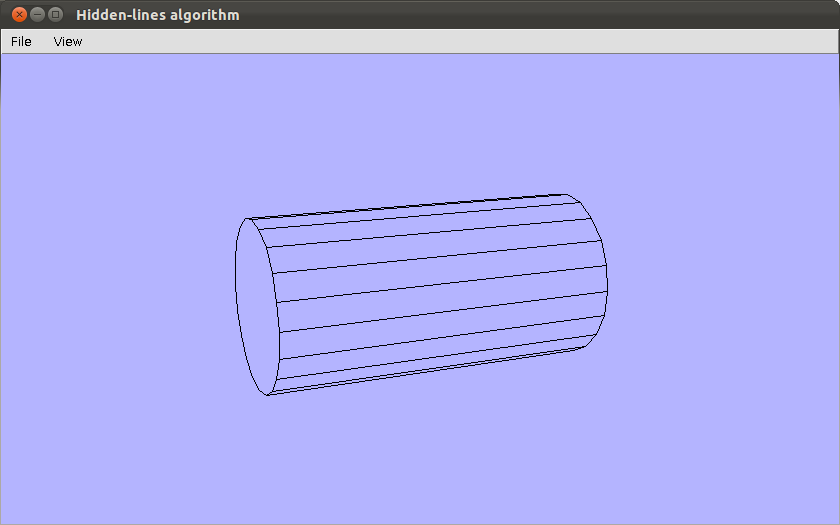
A simple rendering is to draw a line around the edges of each face in the object. This would be called wire-frame rendering. A slightly more complex rendering is to ensure that lines are hidden if a face falls in front of that line. This is called hidden-line elimination. A cylinder is displayed here as rendered with hidden line elimination:

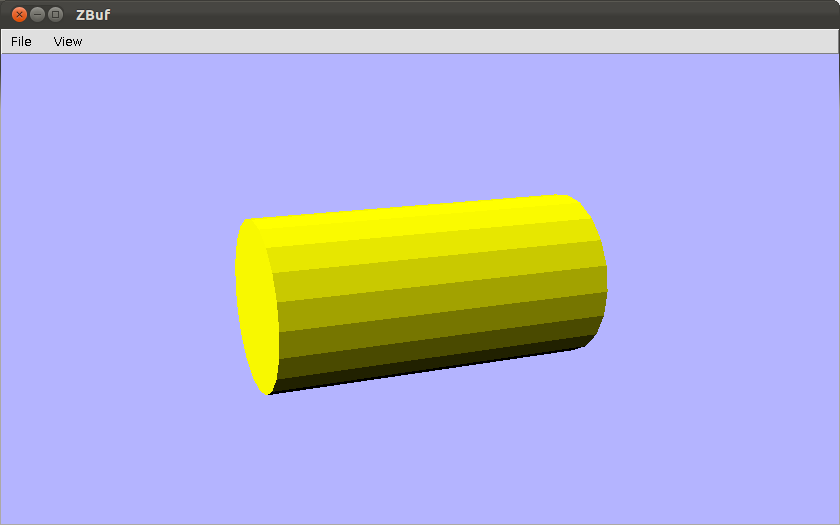
A more realistic rendering gives a color to each face and fills it in. The face’s color can be shaded according to the direction the face makes with a light source. One simple method of rendering these shaded faces is called z-buffering. Here’s a screenshot of a z-buffer rendering of the same cylinder:

What I learned from Evolutionary Computing

875 lines of code and 55 hours. Evolutionary Computing was one of the most challenging courses I have taken at SCSU. These statistics come from our final project, which was a month-long research project. Our assignment was to build on previous projects and produce a 5-page paper suitable for publication at a conference.

I learned a lot while completing this project. My project studied spanning trees on complete graphs, and how to evolve them using a genetic algorithm. Maybe in a follow-up post I’ll introduce these concepts. For now, I want to show what I learned while writing those 875 lines of Python code.

Write a testing function for non-trivial tests. I was checking something by hand, and thought my program wasn’t working. Then I ended up spending several hours debugging something that was not in fact a bug.
Dropbox is an automated version control. Several times I used it to retrieve an old version of a file that I had not committed. This came in very handy.
In vim, you can do :edit! to reload a file from disk. (documentation here)
Time estimating is important when running your jobs on other people’s machines.
I learned how to profile code using cProfile. On Ubuntu, cProfile can be found in package python-profiler.

Git

In git, you can choose to commit only certain changes in a file. It can be done by using git gui. The GUI basically shows you the output of git diff for the changed files in your repo, and you can right click on a line in the diff and choose “Stage Line For Commit.”

I only used this a few times, but it is a lot better than doing the following:

$ cp dandelion.tex dandelion.tex.bak
$ git checkout -- dandelion.tex
$ #manually copy over the changes that you do want to commit
$ git add dandelion.tex
$ git commit -m "This is the hard way"

LaTeX

When writing tables in LaTeX, you must put the label in the caption in order for it to refer to a specific table number. If you don’t, your ref will only refer to the number of the section. Here is a working code snippet:

The times can be seen in Table ref{wallclock}.

begin{table}
caption{Wall clock times in seconds for a single
run of the genetic algorithm using the PyPy interpreter.
 label{wallclock}
}
begin{tabular}{l r}
...
end{tabular}
end{table}

bobbyratliff

Creating structures that automate things people do every day.